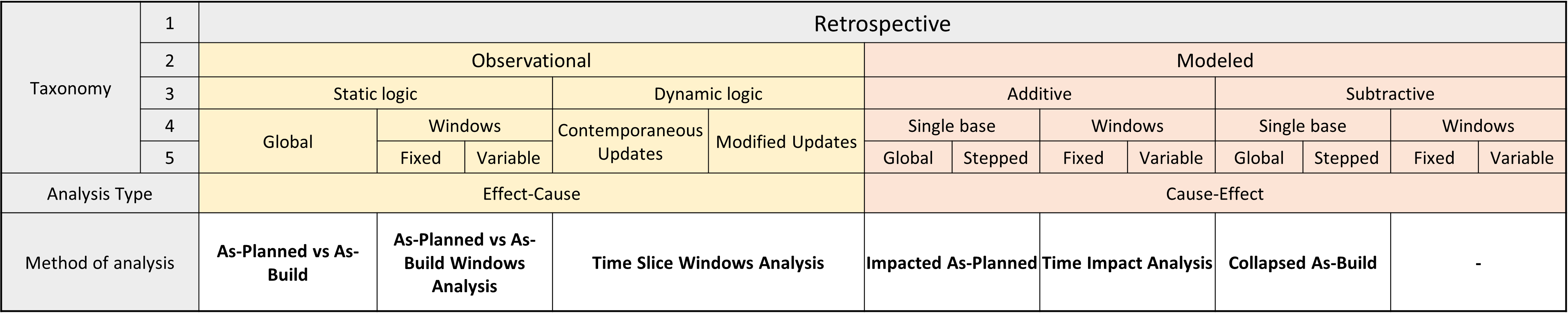
The classification of delay analysis methods combines the taxonomic classification conducted by the AAEC with the six main methods of the SCL. It’s important to note that specific implementations can be applied for each method, giving rise to variations within the same method.
Level 1: Time
At the first hierarchical level, the analysis is categorized based on the moment it is carried out, resulting in two branches: prospective and retrospective.
Prospective Analysis: This approach involves making estimates about future events, and the analysis occurs while the project is still in progress, rather than in a “forensic” context.
Retrospective Analysis: In contrast, retrospective analysis is conducted after the delay has occurred, and its impact is known. The As-Built documentation is a crucial source of information for the application of delay analysis methods in retrospective scenarios, as it provides comprehensive data on the actual project status.
Level 2: Basic Methods
The second hierarchical level consists of two branches: observation and modeling. These basic methods differ in their approach to analyzing delays.
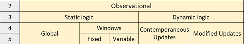
Observation Method: This method involves analyzing the project schedule without making any changes to it. The focus is on comparing the planned schedule with the actual progress to identify delays.
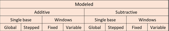
Modeling Method: Unlike the observation method, the modeling method requires active intervention from the analyst. It involves using specialized software like Primavera P6 or MS Project to create simulations and evaluate the impacts of delays. The analyst may insert or extract activities in the schedule to assess various scenarios and compare the calculated results.
By combining the AAEC’s time-based classification with the SCL’s observation and modeling approaches, a comprehensive framework for classifying delay analysis methods is established. This taxonomy provides a foundation for selecting and applying appropriate delay analysis techniques based on the project’s specific context and available data.
Level 3: Specific Methods
Observational
Within the observation method, two distinctions are made based on the type of evaluation: static logic observation and dynamic logic observation.
- Static Logic Observation: The term “static” refers to the original planning, which remains unchanged from the beginning of the project. This method involves comparing an As-Planned schedule with an As-Built schedule for the same project.
- Dynamic Logic Observation: The term “dynamic” refers to the relationships that vary during project execution. In this method, updated schedules are used to reflect the progress of the work and any sequence changes or strategies that deviate from the baseline.
Modeled
In the modeling method, two distinctions are made based on how delays are treated during analysis: additive modeling and subtractive modeling.
- Additive Modeling: In additive modeling, a schedule is compared with another schedule in which elements have been inserted to model a specific scenario.
- Subtractive Modeling: In subtractive modeling, the As-Built schedule is compared with another schedule where elements have been removed to model a certain scenario.
Level 4: Basic Implementations
The fourth hierarchical level includes two implementations for each of the Level 3 clusters.
Static Logic Observation Implementation:
- Global: Considers the entire duration of the project as a single period for analysis.
- Periodic (Windows): Segments the project into various periods (windows) and analyzes each period separately. These windows are static logic and do not account for changes in sequence or strategy that occurred throughout the project.
Dynamic Logic Observation Implementation:
- Contemporary Updates: Evaluates each update without altering or modifying anything. It reflects the dynamic changes in the project schedule without interference.
- Recreated Updates: In this implementation, the analyst modifies the schedule to correct errors, adjust to reality, or recreate it entirely in the absence of updated schedules.
Additive and Subtractive Modeling Implementation:
- Single base: Involves using a single schedule with a specific sequence or set of updates for analysis.
- Multi base (windows): Utilizes multiple schedules with different updates to explore various scenarios.
By understanding these specific methods and their implementations, delay analysis can be effectively carried out to identify and address project delays with greater accuracy and clarity.
Level 5: Specific Implementations
At the last level, specific implementations are categorized based on the use of windows or segments and the application of simple modeled methods. This level distinguishes between the following:
Fixed Periods vs. Variable Periods:
- Fixed Periods: In this implementation, the analysis is conducted on specific schedule update dates, usually at regular intervals such as months or weeks. Each updated period is analyzed separately, allowing for a more focused examination of individual progress stages.
- Variable Periods: Contrary to fixed periods, variable periods are established based on changes in the critical path or new schedule revisions. This approach accommodates shifts in project dynamics and considers unique periods dictated by significant alterations in the project’s course.
Global vs. Step by Step
This specific implementation pertains to the additive and subtractive modeling methods.
- Global: In the global application, delays are inserted or removed in a single operation across the entire schedule. This method offers an overview of the overall impact of delays, simplifying the analysis process.
- Step by Step: In contrast, the step-by-step application involves the sequential inclusion or removal of delays. For the additive modeling method, this typically means adding delays from the initial activity to the final activity of the project (push case). Conversely, in the subtractive modeling method, delays are removed starting from the final activity and progressing backward to the project’s start activity.
By understanding and applying these specific implementations, delay analysis becomes more specific and tailored to the project, providing valuable insights into project performance and potential areas for improvement.